Building Transformer Models for Proteins From Scratch

A Practical Guide to Building and Evaluating Protein Language Models

Introduction

Building on our understanding of protein science foundations from the previous article, we're now ready to explore the exciting intersection of AI/ML and protein science. This article focuses on transformer-based language models, the technology powering advanced chatbots like ChatGPT. I won't spend too much space on the in-depth explanations of transformers. For that, I highly recommend the blog post "The Illustrated Transformer" by Jay Alammar, which provides a detailed breakdown and beautiful illustrations. Instead, we'll focus on the practical implementation of transformers for protein analysis.

Specifically, we will build a basic protein transformer model to predict the antigen specificity of antibody sequences. This project will enhance our understanding of transformer implementation and their potential applications within protein science.

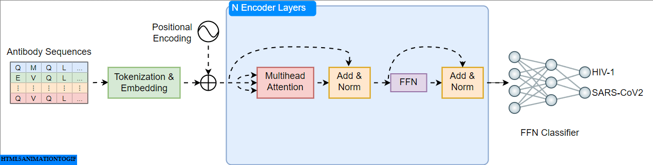
Transformers, introduced in the groundbreaking paper "Attention Is All You Need" are neural networks with encoder and decoder components. Models like BERT (Bidirectional Encoder Representations from Transformers) leverage the encoder for understanding language and excel at downstream tasks like classification. Here, we'll implement and train an encoder-based model to classify antibodies as HIV-1 or SARS-CoV-2 specific (Figure 1).

Figure 1. Overview of the transformer-based antibody classifier.

Code

Throughout the article, I'll provide code snippets for demonstration and clarity. For the complete, documented code and scripts, please refer to the GitHub repository for this article.

Data

For this project, I've collected a dataset of several hundred BCRs (B cell receptor) or antibodies from the IEDB, specifically targeting either HIV-1 or SARS-CoV-2. The goal is to train a transformer model to perform binary classification, predicting which antigen an antibody sequence binds to.

Figure 2. Balanced HIV-1 and SARS-CoV-2 classes in the dataset

The dataset has been initially split into a training set and a hold-out test set. During model training and tuning, the training set will be further divided into a smaller training subset and a validation subset. The processed datasets are available for download in the data directory of the GitHub repo, and the preprocessing steps are detailed in the notebooks/bcr_preprocessing.ipynb notebook. We will implement a custom PyTorch Dataset class as below to load and prepare data for our model:

  class BCRDataset(Dataset):

    def __init__(self, df: pd.DataFrame):
        super().__init__()
        self.df = df

    def __len__(self) -> int:
        return len(self.df)

    def __getitem__(self, i) -> tuple[str, int]:
        x = self.df.loc[i, "sequence"]
        y = self.df.loc[i, "label"]
        return x, y 

This code defines the BCRDataset class, a custom dataset designed for working with antibody data stored in a Pandas DataFrame. The class includes functions to initialize the dataset with a DataFrame (__init__), return the total number of samples (rows) in the DataFrame (__len__), and retrieve a single data sample by index (__getitem__). The __getitem__ function is responsible for extracting the amino acid sequence ('sequence') and its associated label ('label') from the DataFrame and returning them as a tuple.

During training, this dataset class will be used to fetch and preprocess batches of data efficiently. The dataset will then be delivered to the model by a customized DataLoader that manages how the data is batched and loaded onto the GPU (if available) for training.

Tokenization

Transformers don't directly process raw text or protein sequences. Instead, the input is first broken down into tokens. In protein analysis, we tokenize a protein sequence into its individual amino acids. Each amino acid, along with special tokens for the start, end, padding, and unknown symbols, is then assigned a unique integer value. This process translates the protein sequence into a numerical representation that the transformer model can understand.

Here's the essential code for this tokenization step:

class Tokenizer:

    def __init__(self):
        # special tokens
        vocab = ["<cls>", "<pad>", "<eos>", "<unk>"]
        # 20 anonical amino acids
        vocab += list("ACDEFGHIKLMNPQRSTVWY")
        # mapping
        self.token_to_index = {tok: i for i, tok in enumerate(vocab)}
        self.index_to_token = {i: tok for i, tok in enumerate(vocab)}

    def __call__(
        self, seqs: list[str], padding: bool = True
    ) -> dict[str, list[list[int]]]:
        """
        Tokenizes a list of protein sequences and creates input representations with attention masks.
        """

        input_ids = []
        attention_mask = []

        if padding:
            max_len = max(len(seq) for seq in seqs)

        for seq in seqs:
            # Preprocessing: strip whitespace, convert to uppercase
            seq = seq.strip().upper()

            # Add special tokens
            toks = ["<cls>"] + list(seq) + ["<eos>"]

            if padding:
                # Pad with '<pad>' tokens to reach max_len
                toks += ["<pad>"] * (max_len - len(seq))

            # Convert tokens to IDs (handling unknown amino acids)
            unk_id = self.token_to_index["<unk>"]
            input_ids.append([self.token_to_index.get(tok, unk_id) for tok in toks])

            # Create attention mask (1 for real tokens, 0 for padding)
            attention_mask.append([1 if tok != "<pad>" else 0 for tok in toks])

        return {"input_ids": input_ids, "attention_mask": attention_mask}

The Tokenizer utilizes special tokens such as <cls>, <eos>, and <pad> to denote the beginning, end, and any padding within the protein sequences. It also handles unexpected amino acids by employing an <unk> token. During initialization (__init__), the vocabulary is built, establishing mappings between amino acids, special tokens, and their corresponding numerical representations. The core tokenization process occurs within the __call__ function, where special tokens are added, sequences are converted into lists of integer IDs, and padding is optionally applied for uniform input lengths.

Embedding and Positional Encoding

After tokenization, we use an embedding layer to convert the integer values representing our amino acids into vectors of floating-point numbers called embeddings. Embeddings can be considered as coordinates within a high-dimensional space. During training, the model learns to position similar amino acids closer together within this space (Figure 3).

Figure 3. Example amino acid embeddings and their visualization in 3D space

The order of amino acids determines the primary sequence of protein sequences. However, transformer models lack an inherent understanding of sequential position. To address this, we use positional encoding. Positional encodings are special signals added to the amino acid embeddings, informing the model about the relative position of each amino acid within the protein sequence. As shown in Figure 4, this results in a unique encoding pattern at each position within the sequence.

Figure 4. Positional encoding

Self-attention

After tokenization, our amino acid integers are converted into embedding vectors. Each of these embeddings is then used to generate three new vectors through linear transformation: a query (q), a key (k), and a value (v). These vectors are essential for calculating scaled dot-product attention, the core mechanism that enables self-attention within transformers. The scaled dot-product attention formula is as follows:

\(\text{Softmax}\left(\frac{\mathbf{q}\mathbf{k}^\intercal}{\sqrt{d_k}}\right)\mathbf{v}\)

The query vector of each token is compared to the key vectors of all tokens in the sequence (including itself) using dot products. Dot products measure similarity, so a higher dot product suggests a stronger relationship between the tokens. To improve stability, we scale these dot products by the square root of the embedding dimension (dk). We also have the option to mask out certain tokens if needed.

A softmax function is applied to the dot products, giving us attention scores. These scores tell us how much each token should "attend to" the other tokens in the sequence.

Finally, for each token, we calculate a new representation by summing the value vectors (v) of all tokens, weighted by their respective attention scores. This means that the most relevant amino acids in the sequence will have a greater influence on the token's new representation. Let's take a look at how we can implement this in code:

def scale_dot_product_attention(
    q: torch.Tensor, k: torch.Tensor, v: torch.Tensor, mask: torch.Tensor = None
) -> tuple[torch.Tensor, torch.Tensor]:
    """
    Implements scaled dot-product attention, a core component in transformer architectures.
    """

    dk = q.shape[-1]
    attn_logits = q @ k.transpose(-2, -1) / np.sqrt(dk)

    if mask is not None:
        # Mask out with a very large negative value
        attn_logits.masked_fill_(mask == 0, -1e9)

    attention = torch.softmax(attn_logits, dim=-1)
    values = attention @ v

    return values, attention

Unlike previous RNN models, transformers calculate these attention relationships for all tokens in parallel using matrix multiplication. This fully utilizes the power of GPUs, leading to significant improvements in speed and efficiency.

Multi-head attention

While self-attention provides a powerful mechanism for capturing relationships between amino acids within a protein sequence, multi-head attention takes this concept further.  It employs multiple self-attention mechanisms in parallel, allowing each "head" to focus on different aspects of the input. This gives the model the ability to capture diverse relationships and nuances within the protein sequence.  The outputs from multiple heads are then combined, leading to a richer representation of each token.  Importantly, like single-head self-attention, transformers leverage matrix multiplications to compute multiple attention heads simultaneously, maintaining the computational efficiency of the model. Below is a simplified excerpt of how this is implemented:

class MultiheadAttention(nn.Module):
    # ... (other parts of the class) 

    def forward(
        self, x: torch.Tensor, mask: torch.Tensor = None, return_attention: bool = False
    ) -> torch.Tensor:
        """
        Performs multi-head attention on the input.
        """

        batch_size, seq_len = x.shape[0], x.shape[1]

        x = self.input(x)

        # split heads
        x = x.reshape(batch_size, seq_len, self.num_heads, 3 * self.head_dim)

        # swap dims
        x = x.permute(0, 2, 1, 3)

        # q, k, v
        q, k, v = x.chunk(3, dim=-1)

        # expand mask to 4D if needed
        if mask is not None:
            mask = self.expand_mask(mask)

        # Perform scaled dot-product attention
        # values: (batch_size, num_heads, seq_len, head_dim)
        # attention: (batch_size, num_heads, seq_len, seq_len)
        values, attention = scale_dot_product_attention(q, k, v, mask=mask)

        # change dims
        values = values.permute(
            0, 2, 1, 3
        )

        # concat heads
        values = values.reshape(
            batch_size, seq_len, -1
        )

        # output linear layer
        out = self.output(values)

        if return_attention:
            return out, attention

        return out

This code snippet showcases the core functionality of the multi-head attention mechanism. The x = self.input(x) line projects the input sequence into a higher dimensional space, allowing the creation of separate representations for queries (what the model focuses on), keys (used for relevance scoring), and values (the actual information to be extracted). The subsequent lines split the projected input across multiple heads (self.num_heads) and rearrange it for efficient multi-head computations. Finally, the code extracts the individual queries, keys, and values (q, k, v) which are crucial elements for performing attention calculations within the Transformer architecture.

Encoder Layer and Encoder

We can now build upon our multi-head attention implementation to create encoder layers, the building blocks of a transformer encoder. Each encoder layer includes a multi-head attention mechanism to capture relationships between amino acids within a protein sequence, followed by a fully-connected feed-forward network (FFN) layer for further processing.  Additionally, residual connections and layer normalization techniques are employed within each layer to improve training stability and performance.

Here's how an encoder layer can be implemented:

class EncoderLayer(nn.Module):
    # ... (other parts of the class) 

    def forward(self, x: torch.Tensor, mask: torch.Tensor = None) -> torch.Tensor:
        """
        Passes the input sequence through the encoder block.
        """

        #  Multi-head attention layer
        attn_out = self.attention(x, mask)

        # residual connections
        x = x + self.dropout(attn_out)
        # layer norm
        x = self.norm1(x)

        # feed forward
        ffn_out = self.ffn(x)
        # residual connections
        x = x + self.dropout(ffn_out)
        # layer norm
        x = self.norm2(x)

        return x

By stacking multiple encoder layers, the model can learn increasingly complex and hierarchical representations of the protein sequence. The encoder's forward function coordinates the passage of the input sequence through each of its stacked encoder layers. In each layer, the multi-head attention and feed-forward network progressively refine the representation of the protein sequence. The output of the final encoder layer is a highly informative encoded representation ready to be used for downstream tasks.

class Encoder(nn.Module):
    # ... (other parts of the class)

    def forward(self, x: torch.Tensor, mask: torch.Tensor = None) -> torch.Tensor:
        """
        Passes the input sequence through all encoder layers.
        """

        for layer in self.layers:
            x = layer(x, mask)

        return x

The Classification Model

Now we can complete the model for antibody classification using the transformer encoder we've built. The model works as follows: First, as with previous steps, we embed our amino acid tokens into numerical representations and add positional encoding signals.  The encoder, the core of our model, then processes these sequence embeddings and learns complex relationships between amino acids. To obtain a single representation of the entire antibody sequence, we average the outputs of the encoder for each token. Finally, a FFN process this averaged sequence representation and outputs a single value (or logit) to predict the antibody class.

class AntibodyClassifier(nn.Module):
    # ... (Class definition, omit __init__ and mean_pooling for brevity) 

    def forward(self, batch: dict[str, torch.Tensor]) -> torch.Tensor:
        """Forward pass through the model."""

        input_ids, attention_mask = batch["input_ids"], batch["attention_mask"]

        # map tokens to vectors
        x = self.embedding(input_ids)

        # add positional encoding
        x = self.pe(x) 

        # pass through the Transformer encoder for sequence processing
        x = self.encoder(x, attention_mask)

        # Mean pooling
        x = self.mean_pooling(x, attention_mask)

        # Classification head
        logits = self.classifier(x)

        return logits

The forward function outlines the step-by-step process of transforming an input antibody sequence into a class prediction (e.g., HIV-1 or SARS-CoV-2). First, the model embeds the amino acid tokens and adds positional information. Next, the heart of the model – the transformer encoder – processes this sequence representation, learning complex relationships within the protein. To obtain a single vector representing the entire sequence, mean pooling is applied, taking into account the attention mask. Finally, a feed-forward classification head takes this pooled representation and generates logits (unnormalized probabilities) for each antibody class.

Model Training

The next step is to train our antibody classifier using the HIV-1 and SARS-CoV-2 data we prepared earlier. To train the model, run the train.py script from the root directory of the project repo using your terminal. This script offers various customizable parameters to control the training process. For example, to execute the training script with default parameters and store the results under a run ID named train01, use the following command:

python protein_transformer/train.py --run-id train01 --dataset-loc data/bcr_train.parquet 

Here are some key default hyperparameters:

embedding_dim = 64: Dimensionality of token embeddings.
num_layers = 8: Number of encoder layers.
num_heads = 2: Number of attention heads in the encoder.
ffn_dim = 128: Dimensionality of the feed-forward layer in the encoder.
dropout = 0.05: Dropout rate for regularization.

During training, monitor both the training loss and validation loss. Ideally, both should decrease over epochs. A plot of these losses versus epochs can provide valuable insights into the training process (Figure 5).

Figure 5. Training and validation loss

Upon completion, the script stores training results in the runs/train01 directory by default. This includes model arguments, the best-performing model (based on validation loss), training and validation loss records, along with validation metrics for each epoch. These metrics, which include the following, are saved in the runs/train01/results.csv file:

Accuracy: 0.727
AUC score: 0.851
Precision: 0.734
Recall: 0.727
F1-score: 0.725

We can potentially improve our model's performance even further by exploring different hyperparameter combinations. We'll cover hyperparameter tuning in the next section.

Hyperparameter Tuning

To improve the performance of our antibody classifier, we'll explore hyperparameter tuning with Ray Tune, which allows us to efficiently run trials in parallel. Here's the search space we'll investigate:

embedding_dim: Values of 16, 32, 64, or 128.
num_layers: Values ranging between 1 and 8.
num_heads: Values of 1, 2, 4, or 8.
dropout: Values between 0 to 0.2, with increments of 0.02.
lr (learning rate): Values between 1e-5 and 1e-3 (log-uniform distribution).

To initiate the tuning process with default parameters and store the results under a run ID named tune01, execute the tune.py script from the project root directory:

python protein_transformer/tune.py --run-id tune01 --dataset-loc /home/ytian/github/protein-transformer/data/bcr_train.parquet

By default, it will execute 100 trials with different parameter combinations, running each trial for up to 30 epochs. Ray Tune utilizes early stopping for unpromising trials, allowing for efficient exploration of the hyperparameter space and focuses resources on better-performing configurations. It will track the results of each trial, and upon completion, the best-performing model based on validation loss will be saved in the runs/tune01 directory by default. Additionally, tuning logs, including results from each trial, are stored within the same runs/tune01 directory for easy access and analysis.

Model Evaluation

Now it's time to assess the performance of our best-performing model from the hyperparameter tuning process on the hold-out test dataset. This dataset was kept separate during training and tuning, ensuring that our evaluation reflects true generalization ability.

For example, to evaluate the best model from the tune01 run, execute the following command from the command line:

python protein_transformer/evaluate.py --run-dir runs/tune01 --dataset-loc /home/ytian/github/protein-transformer/data/bcr_test.parquet

Upon completion, the script will save test metrics in a file named test_metrics.json, like the following example, within the run directory provided in the evaluate.py command:

Accuracy: 0.761
AUC score: 0.837
Precision: 0.761
Recall: 0.761
F1-score: 0.761

To gain a deeper understanding of our model's performance, we'll examine two key visualizations: the confusion matrix and the ROC (Receiver Operating Characteristic) curve. The confusion matrix breaks down the model's predictions into true positives, true negatives, false positives, and false negatives, providing insights into where the model excels and where it might struggle. The ROC curve illustrates the model's ability to discriminate between classes at different decision thresholds, with the overall area under the curve (AUC) indicating its effectiveness.

As shown in Figure 6, the confusion matrix demonstrates a balanced distribution for both HIV-1 and SARS-CoV-2 classes, indicating the model's ability to correctly classify the majority of samples. The ROC curve further supports this, demonstrating a good overall ability to distinguish between the classes (AUC score of 0.84), indicating strong performance that significantly surpasses a random model.

Figure 6. Normalized confusion matrix and ROC curve

Summary

In this blog post, we've explored the practical aspects of building a transformer-based model for antibody classification. We started by collecting and preprocessing antibody sequence data from HIV-1 and SARS-CoV-2 datasets.  Next, we tokenized these sequences, converted them into numerical representations (embeddings), and built an encoder architecture using transformer layers. To make predictions, we added a classification head on top of the encoder. We then trained the model, explored hyperparameter tuning with Ray Tune to improve performance, and finally, evaluated our best model on a hold-out test set using metrics like accuracy, AUC score, precision, recall, and F1-score.

Future Work

Although the transformer model we implemented here is relatively simple, it demonstrates the potential of these models in protein science. Indeed, several transformer-based protein language models (PLMs), such as ESM-2, have been pretrained on millions of protein sequences and can be adapted for various downstream tasks such as predicting protein properties and structures. We will continue exploring this exciting area in future posts.

Acknowledgments

• IEDB

• UvA Deep Learning

• Made With ML